The standard error SE of log10(N) is used to adjust the fatigue life or the damage predicted to any given probability of survival. Fatigue life data always include some scatter, and at any given level of stress, the distribution of fatigue lives is assumed to be a log-normal distribution. Or stated differently, a Normal or Gauss distribution of the logarithm of the fatigue life.
The standard error
In practice, if we want to make a life or damage prediction based on a particular percentage probability of survival, we use a lookup table (see Table 1 below) to determine the deviation from the mean (50%) life in terms of the number of standard errors.
The values in the table are calculated using the Probability Density Function (PDF) and the Cumulative Density Function (CDF) of the normal distribution.
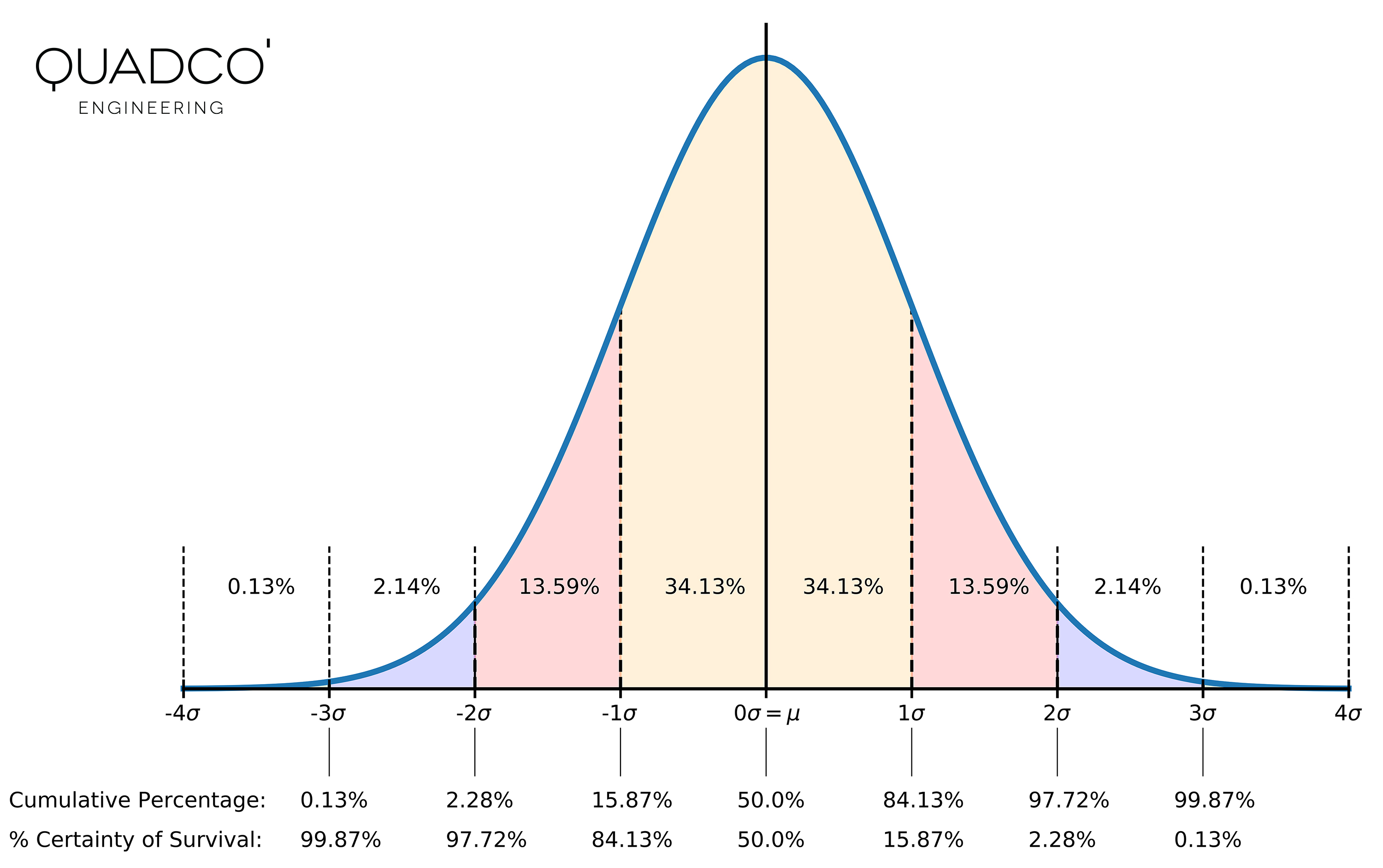
The Probability Density Function (PDF) is the normal distribution curve shown in Figure 1 below:
$${\displaystyle {\frac {1}{\sigma {\sqrt {2\pi }}}}\;\exp \left(-{\frac {\left(x-\mu \right)^{2}}{2\sigma ^{2}}}\right)}$$
With:
- $\mu$ the mean of the data
- $\sigma$ the standard deviation of the mean
The Cumulative Density Function is the integral of the PDF:
$${\displaystyle {\frac {1}{2}}\left(1+\mathrm {erf} \,{\frac {x-\mu }{\sigma {\sqrt {2}}}}\right)}$$
The percentage certainty of survival is then 1 - CDF (see also Figure 1).
| Number of SD's from the mean |
% Certainty Of Survival |
|---|---|
| -5 | 99.99997 |
| -4 | 99.997 |
| -3 | 99.87 |
| -2 | 97.72 |
| -1 | 84.13 |
| 0 | 50 |
| 1 | 15.87 |
| 2 | 2.28 |
| 3 | 0.13 |
| 4 | 0.003 |
| 5 | 0.00003 |
Calculation example
As an example, let's say we have a component which is subject to a cyclic stress with constant amplitude, cycling between ±300 MPa. The component has a material for which we know the parameters of the S-N curve for a certainty of survival of 50%. Those parameters are:
- stress range intercept SRI = 1300 MPa
- the slope of the curve b1 = -0.0612
- standard error SE = 0.12
The above parameters define an S-N curve in terms of the stress range, not the stress amplitude. The stress range Sr is a function of the number of cycles to failure N:
$${\displaystyle S_r = SRI \cdot N^{b_1}}$$
In our case the stress range is 2 ⋅ 300 MPa = 600 MPa. The predicted number of cycles to failure for the component, based on a certainty of survival of 50% S-N curve, will be:
$${\displaystyle 600 = 1300 \cdot N_{50}^{-0.0612}}$$
or N50 = 306760 cycles.
We now want to use the design S-N curve (typically a certainty of survival of 97.7% is used in most designs) and not the mean S-N curve. What is the predicted number of cycles at which the component will fail, based on a certainty of survival of 97.7% S-N curve?
First we need to find out the number of standard deviations n from the mean that corresponds to a certainty of survival of 97.7%. In Table 1 we find n = -2 for a certainty of survival of 97.7%.
The S-N curve is adjusted by shifting the curve to the left, or put differently, by reducing the number of cycles:
$${\displaystyle log_{10}(N) = log_{10}(N_{50}) - n \cdot SE}$$
or expressed in a different way:
$${\displaystyle N = N_{50} \cdot 10^{(-n \text{ } \cdot \text{ } SE)}}$$
$${\displaystyle N_{97} = 306760 \cdot 10^{(-2 \text{ } \cdot \text{ } 0.12)}}$$
This gives us N97 = 176522 cycles, or a reduction of 42% of the fatigue life compared to N50.