The Ramberg-Osgood Equation

The Ramberg-Osgood relationship

Hooke's law states that below the yield point, the stress is linearly proportional to the strain:

$${\sigma = {E} \; {\varepsilon}_{e}}$$

Ramberg and Osgood defined a power-law to describe the plastic strain:

$${{\varepsilon}_{p} = \left(\frac{\sigma}{K} \right)^n}$$

The material dependent parameters $K$ and $n$ describe the hardening behaviour of the material.

The total strain ${\varepsilon}_{t}$ is the sum of the elastic strain ${\varepsilon}_{e}$ and the plastic strain ${\varepsilon}_{p}$, which results in:

$${{\varepsilon}_{t} = {\varepsilon}_{e} + {\varepsilon}_{p} = \frac{\sigma}{E} + \left(\frac{\sigma}{K} \right)^n}$$

With:

• ${\varepsilon}$ the strain
• ${\sigma}$ the stress
• $K$ material nonlinear modulus
• $n$ material strain-hardening exponent

Accuracy of the equation

The equation is not a perfect representation of the real material's stress-strain behaviour, because the Ramberg-Osgood equation implies that plastic strain is present at any stress level, also way below the yield point. However, the plastic strain part of the total strain is very small at low stress levels.

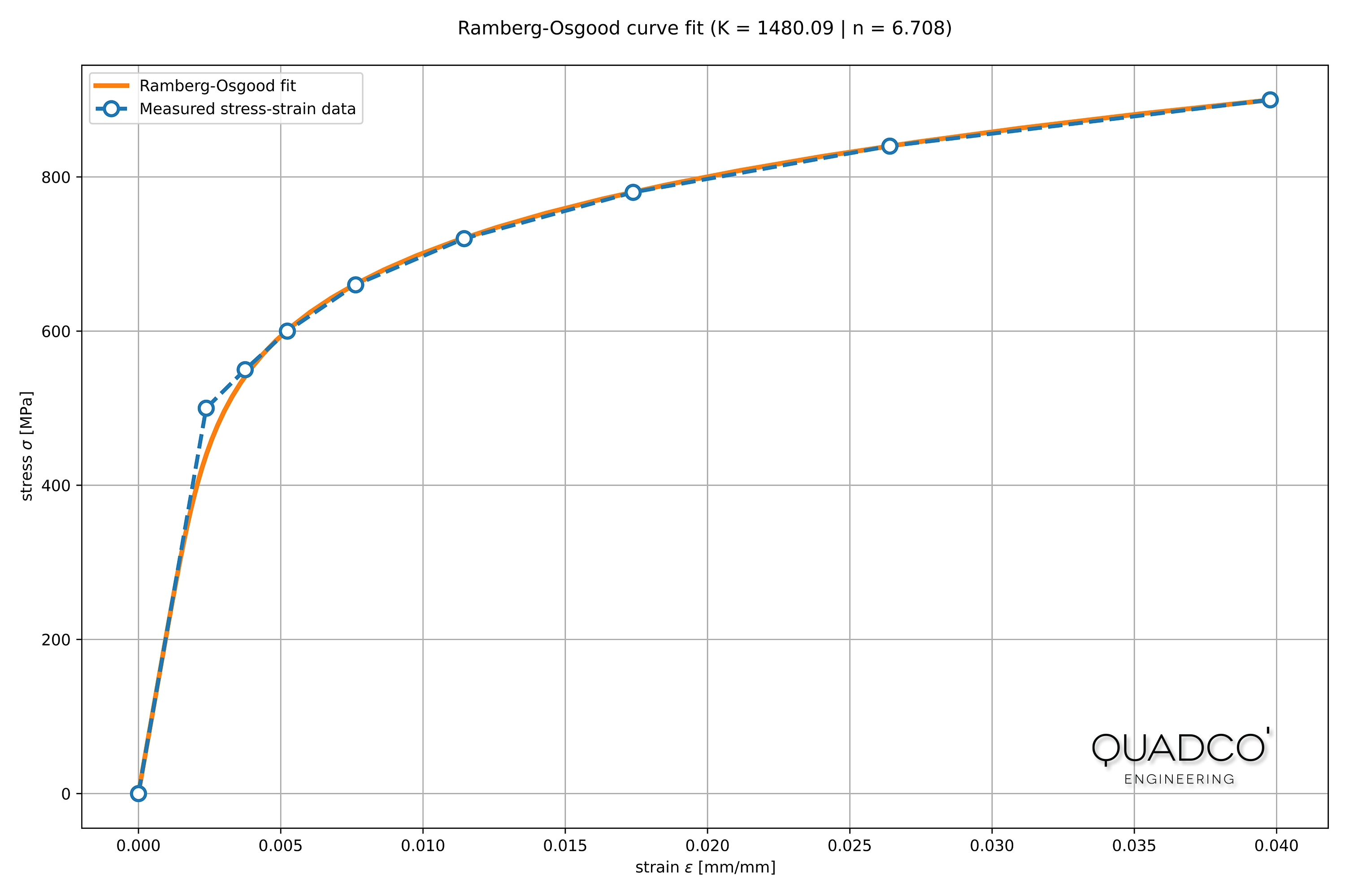
Some materials show an abrupt change of stiffness at yielding. In that case, the Ramberg-Osgood relationship doesn't hold well around the yield point (see Figure 1 below).

Example

In Figure 1, the stress-strain data of a carbon steel with a yield stress σ_y = 500 MPa and a Young's Modulus E = 210000 MPa is presented. The Ramberg-Osgood curve (K = 1480, n = 6.71) is plotted against the measured stress-strain data. The error at stresses between zero and around 350 MPa is very small, but increases at stresses between 400 and 550 MPa.

The Ramberg-Osgood curve provides the material input needed for elastic-plastic FEA calculations, and is equally important for fatigue and durability analysis, where the cyclic stress-strain curve governs the local strain range at notches and stress concentrations.

How to fit stress-strain data to the Ramberg-Osgood equation?

Fitting the stress-strain data to a Ramberg-Osgood curve can be done using Excel, but also with, for example, Python. The Python 3.x code is provided below:

     
import numpy as np
from scipy.optimize import curve_fit
import matplotlib.pyplot as plt


# MATERIAL DATA
strain = np.array([0, 500/210000, 0.003749347, 0.005234888, 0.007631515, 
                   0.011446096, 0.017384888, 0.026405375, 0.039775799])
stress = np.array([0, 500, 550, 600, 660, 720, 780, 840, 900])
E = stress[1] / strain[1]  # CALCULATE YOUNG'S MODULUS

# FITTING RAMBERG-OSGOOD EQUATION
def test_func(x, K, n):
    return x / E + np.power(x / K, n)

p0 = [500, 5]  # Initial estimate for [K, n]
c, cov = curve_fit(test_func, stress, strain, p0)

# PRINT CURVE FIT PARAMETERS
print()
print('-' * 28)
print(' Ramberg-Osgood parameters')
print('-' * 28)
print(f' K = {c[0]} \n n = {c[1]}')
print('-' * 28)

# CREATE DATA ARRAY FOR THE FITTED CURVE
e = test_func(np.linspace(0, stress[-1]), c[0], c[1])  # STRAIN
s = np.linspace(0, stress[-1])  # STRESS

# PLOT DATA AND FITTED CURVE
plt.figure(1, figsize=(12, 8))
# PLOT FITTED CURVE:
plt.plot(e, s, lw=3, c='C1')
# PLOT MEASURED DATA:
plt.plot(strain, stress, '--o', lw=2.5, ms=9, mew=2, mfc='white', c='C0')
plt.grid()
plt.xlabel(r'Strain $\epsilon$ [mm/mm]')
plt.ylabel(r'Stress $\sigma$ [MPa]')
plt.title(f'Ramberg-Osgood curve fit (K = {np.round(c[0], 2)} '
          f'| n = {np.round(c[1], 3)})\n')
plt.legend(['Ramberg-Osgood fit', 'Stress-Strain measured data'])

plt.show()