Certainty of Survival
Fatigue life data always contain scatter. Even carefully controlled laboratory specimens of the same material, tested at the same stress level, will fail at different numbers of cycles. At any given stress, the distribution of fatigue lives is assumed to follow a log-normal distribution — that is, a normal (Gaussian) distribution of log10(N). The standard error SE of log10(N) is the statistical parameter used to shift an S‑N curve from its mean (50 %) survival probability to any other probability of survival required for design.
Why Certainty of Survival Matters
A mean S‑N curve represents the stress-life relationship at which 50 % of specimens would be expected to survive. Designing a component against a 50 % survival probability would mean accepting that half of all parts in service could fail before reaching the predicted life — an unacceptable risk for virtually any engineering application.
In practice, fatigue assessments use design S‑N curves that are shifted to a higher certainty of survival. The most common choices are 97.7 % (mean minus two standard deviations, widely used in general mechanical engineering and codified in guidelines such as the FKM Guideline) and 99.9 % or higher for safety-critical applications such as aerospace, nuclear or railway components. The choice of survival probability is a design decision that balances acceptable risk against the economic cost of a more conservative design.
The Standard Error and the Normal Distribution
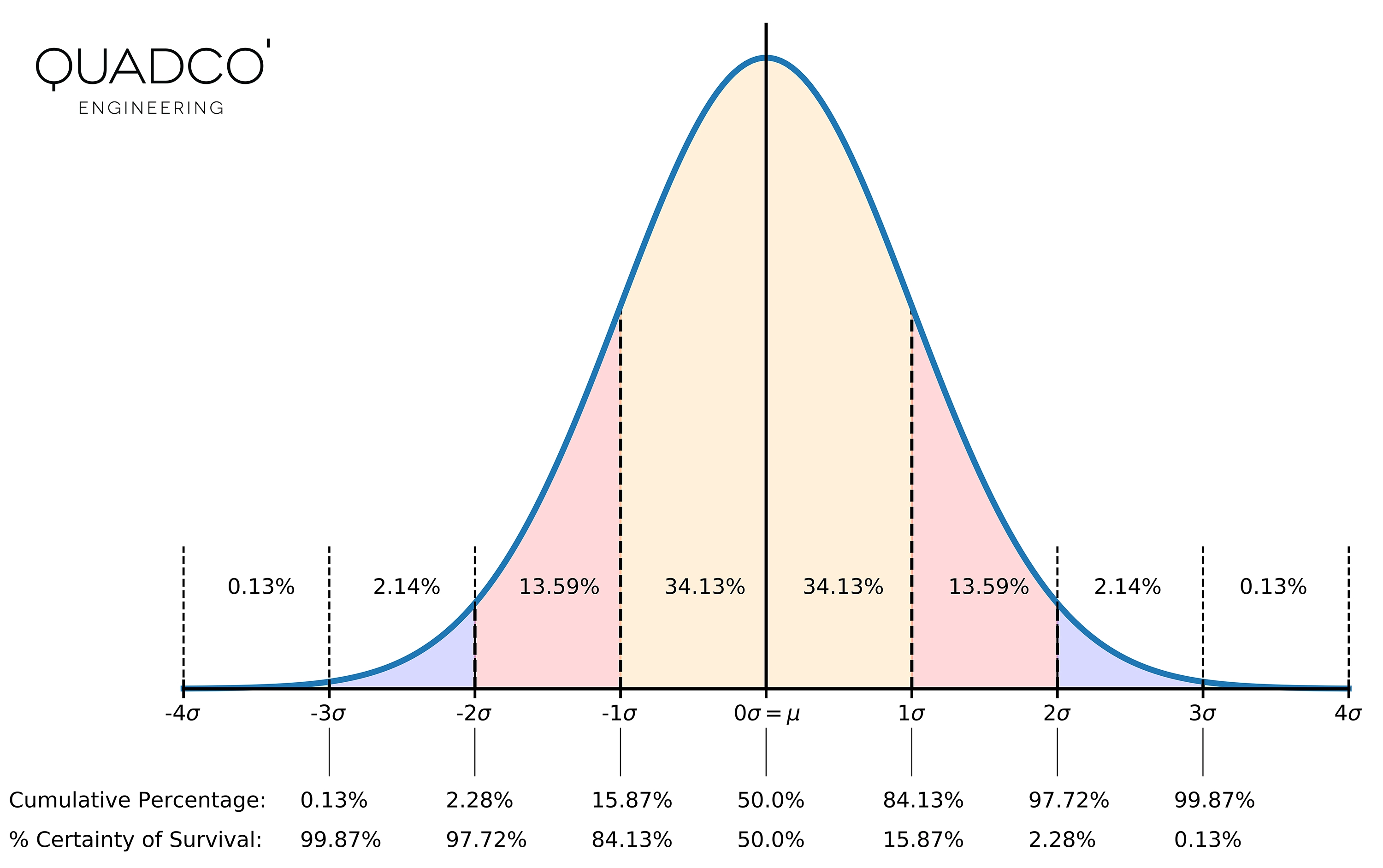
To shift the S‑N curve to a specific probability of survival, we need a lookup table (Table 1) that gives the deviation from the mean life in terms of the number of standard deviations. The values in this table are derived from the Probability Density Function (PDF) and the Cumulative Distribution Function (CDF) of the normal distribution.
The PDF is the familiar bell curve:
$${\displaystyle {\frac {1}{\sigma {\sqrt {2\pi }}}}\;\exp \left(-{\frac {\left(x-\mu \right)^{2}}{2\sigma ^{2}}}\right)}$$
where:
- $\mu$ is the mean of the data
- $\sigma$ is the standard deviation
The CDF is the integral of the PDF:
$${\displaystyle {\frac {1}{2}}\left(1+\mathrm {erf} \,{\frac {x-\mu }{\sigma {\sqrt {2}}}}\right)}$$
The percentage certainty of survival is then 1 − CDF (see also Figure 1).
| Number of SD's from the mean |
% Certainty of Survival |
|---|---|
| −5 | 99.99997 |
| −4 | 99.997 |
| −3 | 99.87 |
| −2 | 97.72 |
| −1 | 84.13 |
| 0 | 50 |
| 1 | 15.87 |
| 2 | 2.28 |
| 3 | 0.13 |
| 4 | 0.003 |
| 5 | 0.00003 |
Calculation Example
Suppose we have a component subjected to constant-amplitude cyclic stress between ±300 MPa. The S‑N curve parameters for this material at 50 % certainty of survival are:
- stress range intercept SRI = 1300 MPa
- slope of the curve b1 = −0.0612
- standard error SE = 0.12
These parameters define the S‑N curve in terms of the stress range (not the stress amplitude). The stress range Sr is a function of the number of cycles to failure N:
$${\displaystyle S_r = SRI \cdot N^{b_1}}$$
The stress range in this case is 2 ⋅ 300 MPa = 600 MPa. The predicted number of cycles to failure at 50 % survival is therefore:
$${\displaystyle 600 = 1300 \cdot N_{50}^{-0.0612}}$$
which gives N50 = 306 760 cycles.
We now want to use the design S‑N curve. In most general engineering applications, a certainty of survival of 97.7 % is used. From Table 1 we find that 97.7 % corresponds to n = −2 standard deviations from the mean.
The S‑N curve is adjusted by reducing the number of cycles:
$${\displaystyle \log_{10}(N) = \log_{10}(N_{50}) - n \cdot SE}$$
or equivalently:
$${\displaystyle N = N_{50} \cdot 10^{(-n \; \cdot \; SE)}}$$
$${\displaystyle N_{97.7} = 306\,760 \cdot 10^{(-2 \; \cdot \; 0.12)}}$$
This gives N97.7 = 176 522 cycles — a reduction of 42 % compared to the mean life N50.
The example illustrates an important point: fatigue scatter is not a minor statistical detail. At 97.7 % survival, the allowable life is less than 60 % of the mean life. When cumulative damage calculations are performed on top of this shifted S‑N curve, the combined effect of scatter and variable-amplitude loading can reduce the predicted safe operating life considerably. This is why the choice of survival probability must be made consciously and documented clearly in every fatigue assessment.
If you want to learn more about fatigue assessment in practice, take a look at our course Introduction to Fatigue Analysis with FEA, which covers S‑N curve usage, survival probability, damage accumulation and the interaction between FEA results and fatigue life prediction.
Frequently asked questions
Common questions about certainty of survival and fatigue scatter.