Surface Roughness Factor K_R

Fatigue tests of specimens are usually done on components with mirror polished surfaces. However, a component with a larger surface roughness will have a reduced fatigue strength. To account for the effect of this surface roughness to the fatigue strength of a material, a roughness factor K_R is used. This surface roughness factor is used to adjust the material S-N curve. This article describes the FKM method for obtaining the surface roughness factor and how to apply this factor to the S-N curve.

FKM surface roughness factor

The FKM-guideline Analytical Strength Assessment defines the roughness factor K_R as follows:

$${\displaystyle K_R=1-a_R \cdot log_{10}(R_Z) \cdot log_{10}\left(\frac {2R_m}{R_{m,N,min}}\right)}$$

With:

• R_Z the surface roughness in µm according to DIN 4768 (see Table 2)
• R_m the tensile strength in MPa
• a_R a constant (see Table 1)
• R_m,N,min the minimum tensile strength in MPa (see Table 1)

The roughness factor K_R = 1 for a polished surface. Surface roughnesses higher than that of a polished surface will have values for K_R < 1.

Table 1 below gives the values for R_m,N,min and for constant a_R for different material types.

Table 2 below provides some indicative values for the surface roughness R_Z of different surface finishes.

Example calculation

As an example, let's look at a steel with a tensile strength R_m = 600 MPa and with a machined surface.

In Table 1 we find for Steel: a_R = 0.22 and R_m,N,min = 400 MPa. Table 2 gives us R_Z = 100 µm for a machined surface.

Putting these values in the above equation gives us:

$${\displaystyle K_R=1-0.22 \cdot log_{10}(100)\cdot log_{10}\left( \frac{2 \cdot 600}{400}\right)} = 0.79$$

Construction of the S-N curve

Before we get to how the S-N curve is adjusted for the surface roughness factor, let's look at how the S-N curve is constructed (see Figure 1 below - click for larger image).

For the number of cycles N_f between 10³ and N_c1 cycles, the S-N curve is defined as:

$${\displaystyle \Delta \sigma(N_f) = SRI_1 \cdot N_f^{b_1}}$$

The stress range Δσ is a function of the number of cycles N_f. SRI1 is the stress range intercept at 1 cycle and b₁ is the slope, which is negative. The parameter N_c1 is called the Fatigue Transition Point and is basically the number of cycles by which a kink in the fatigue curve is noticeable. The value of N_c1 is usually around 10⁶ - 10⁷ cycles.

For N_f > N_c1, the S-N curve is defined as:

$${\displaystyle \Delta \sigma(N_f) = SRI_2 \cdot N_f^{b_2}}$$

SRI₂ is the stress range intercept at 1 cycle and b₂ is the slope, which is negative, for the second part of the S-N curve.

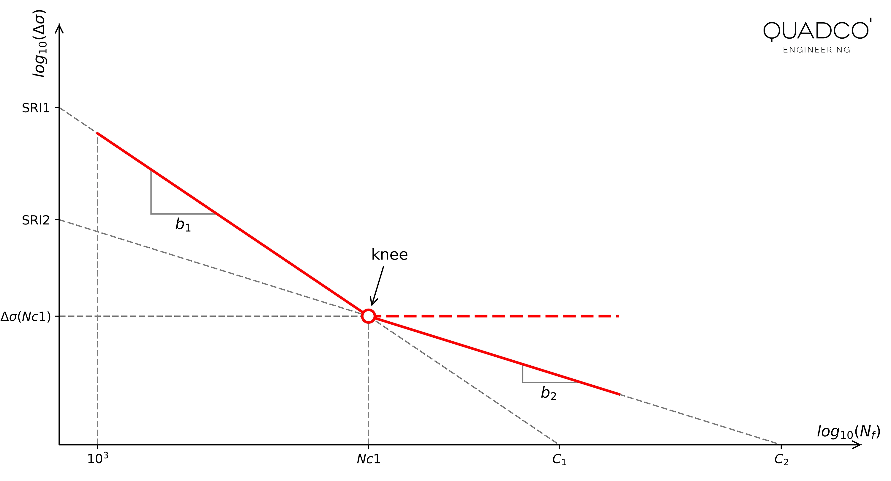
The parameters SRI₁, N_c1, b₁ and b₂ are material parameters derived from the fatigue test data. SRI₂ can be derived as follows:

$${\displaystyle SRI_2 = SRI_1 \cdot (N_{c1})^{b_1-b_2}}$$

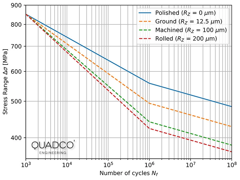
S-N curve adjusted for the surface roughness factor

The surface condition has the greatest effect in the high-cycle regime and becomes progressively smaller towards the low-cycle regime. S-N curves are usually adjusted for the surface roughness by changing the slope b₁ in the first part of the S-N curve (see figure below) and keeping the fatigue strength at 1000 cycles the same. The slope b₂ of the second part of the S-N curve remains unchanged.

So, let's find out how the equation of the S-N curve in Figure 2 is modified. For the unadjusted curve (polished surface), the stress range at N_c1 cycles is:

$${\displaystyle \Delta \sigma(N_{c1}) = 1300 \cdot (10^6)^{-0.0612}=558.14 \text{ MPa}}$$

The stress range Δσ^' at N_c1 cycles for a machined part becomes in our case (with K_R = 0.79, as calculated in the beginning):

$${\displaystyle \Delta \sigma^{'}(N_{c1}) = K_R \cdot 558.14 = 440.97 \text{ MPa}}$$

SRI1^' and b₁^' for the first part of the modified curve can be determined from the two equalities below:

$${\displaystyle SRI1 \cdot (10^3)^{b_1} = 851.81 = SRI_1^{'} \cdot (10^3)^{b^{'}_1}}$$

$${\displaystyle \Delta \sigma^{'}(N_{c1}) = 440.97 = SRI_1^{'} \cdot (10^6)^{b_1^{'}}}$$

When we solve for SRI1^' and b₁^', we find:

$$SRI'_1 = 1645 \; \text{MPa and} \; b'_1 = -0.0953 $$

Since b₂^' = b₂, we can solve below equation for SRI2^':

$${\displaystyle \Delta \sigma^{'}(N_{c1}) = 440.97 = SRI_2^{'} \cdot (10^6)^{b_2}}$$

Which gives us $SRI_{2}^{'} = 677 \text{ MPa}$

The equation of the modified S-N curve between 10³ and N_c1 cycles is then:

$${\displaystyle \Delta \sigma(N_{f}) = 1645 \cdot (N_f)^{-0.0953}}$$

And in the region for N_f > N_c1:

$${\displaystyle \Delta \sigma(N_{f}) = 677 \cdot (N_f)^{-0.0310}}$$