High-Cycle vs. Low-Cycle Fatigue
All fatigue failures share the same basic mechanism — a crack initiates under cyclic loading and propagates until the remaining cross-section can no longer carry the load — but the stress levels, deformation behaviour and analysis methods differ fundamentally between the high-cycle and low-cycle regimes. Understanding which regime applies to a given component is the first step in choosing the right fatigue assessment approach.
High-Cycle Fatigue (HCF)
High-cycle fatigue occurs when a component is subjected to cyclic stresses that remain well below the material's yield strength. Because the deformation is essentially elastic, no significant permanent shape change occurs during any individual cycle. Failure takes a large number of cycles — typically 105 or more — because the crack initiation phase, driven by localised slip bands and micro-crack nucleation, is slow under these low stress amplitudes.
Typical HCF applications include rotating machinery (shafts, gears, bearings), structures subjected to vibration, and any component that accumulates millions of load cycles during its service life.
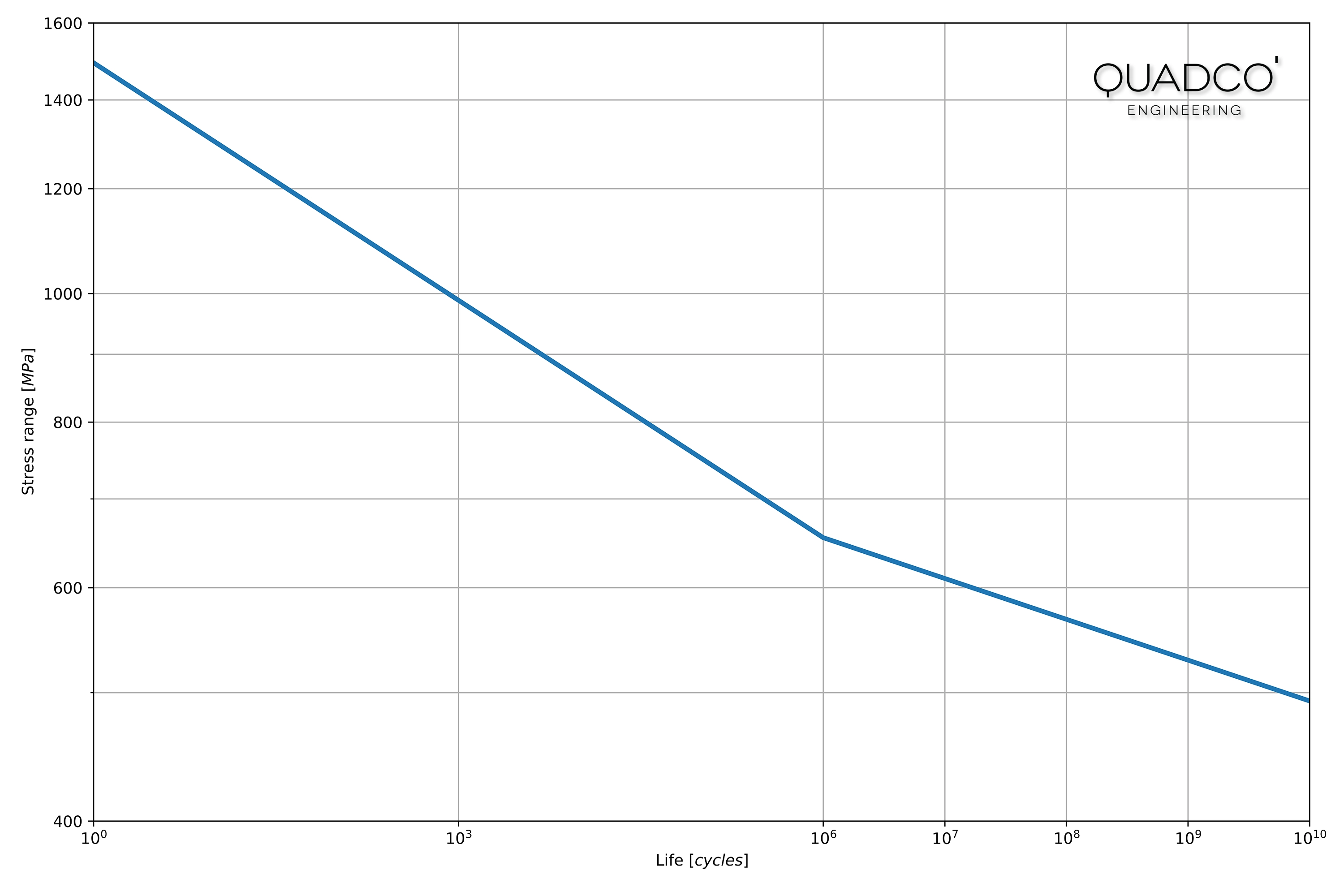
The S‑N curve (stress-life method)
HCF is analysed using the stress-life method, which relates the applied stress range (or amplitude) to the number of cycles to failure via the S‑N curve (also known as the Wöhler curve). Both axes are plotted on a logarithmic scale. The surface roughness factor KR and the certainty of survival adjustment are applied to the S‑N curve to account for real-world conditions.
Low-Cycle Fatigue (LCF)
Low-cycle fatigue occurs when cyclic loads are high enough to cause significant plastic deformation in each cycle, typically at stress levels near or above the yield strength. Under these conditions, the material undergoes permanent shape change every cycle, and failure occurs after a relatively small number of cycles — from as few as a hundred up to approximately 104 cycles.
LCF is common in components subjected to severe thermal cycling (turbine blades, engine exhaust manifolds, pressure vessels during start-up/shutdown) or to high mechanical strain amplitudes (earthquake-resistant structures, landing gear).
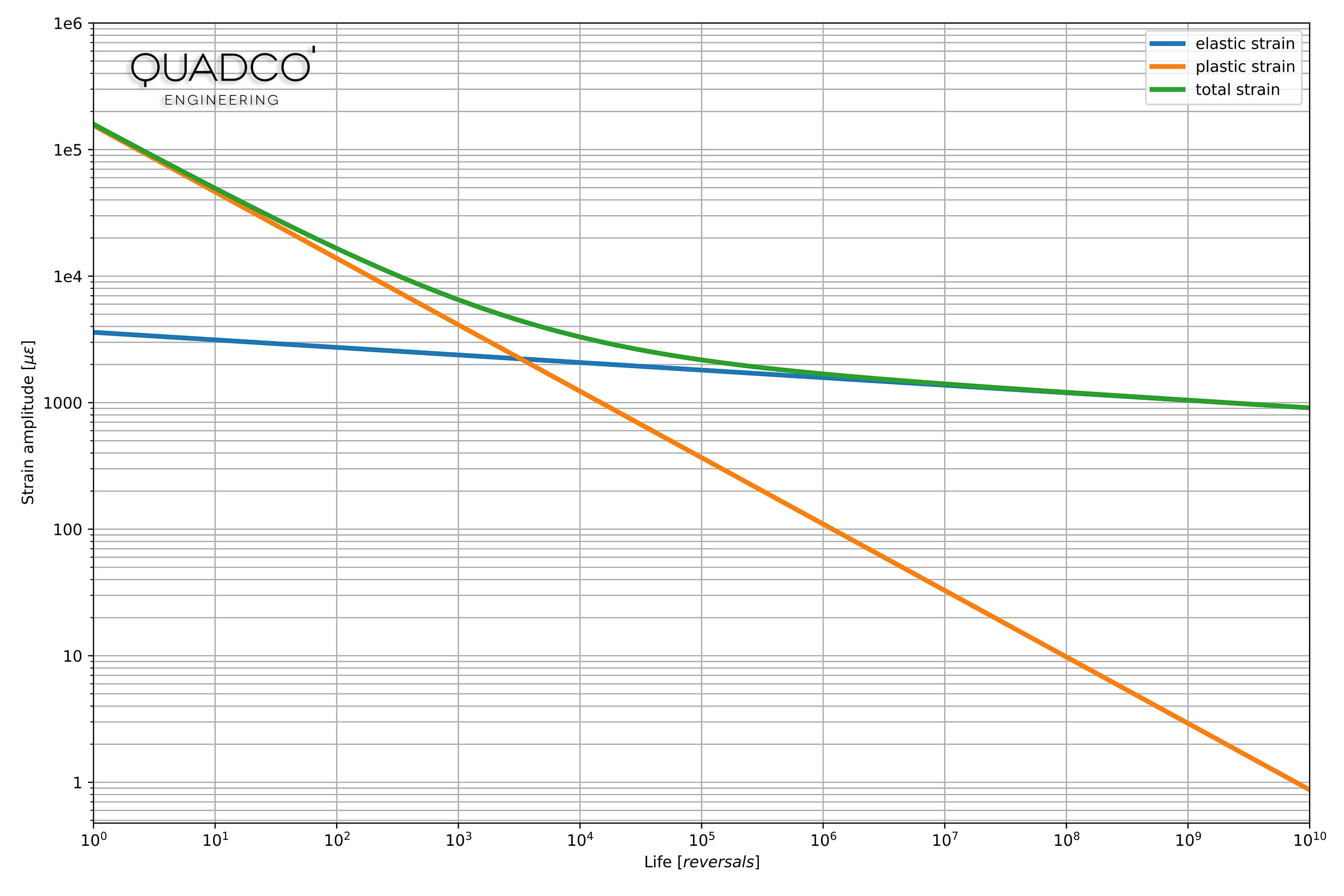
The ε‑N curve (strain-life method)
Because stress alone cannot characterise the cyclic response when the material yields, LCF analysis uses the strain-life method. The ε‑N curve plots the total strain amplitude (elastic plus plastic) against the number of reversals to failure. The Ramberg-Osgood equation is used in conjunction with this curve to describe the cyclic stress-strain relationship of the material, separating the elastic and plastic strain contributions.
Key Differences at a Glance
The boundary between LCF and HCF is not a sharp line at a fixed number of cycles; it is defined by the nature of the material's deformation response. The practical differences that matter for engineers are:
- Stress level and deformation: HCF operates in the elastic regime (stress below yield), while LCF involves macro-plastic deformation at or above yield. This is the defining distinction.
- Cycle count to failure: HCF failures occur after 105 cycles or more; LCF failures typically below 104 cycles. The transition zone between roughly 104 and 105 can exhibit mixed behaviour.
- Analysis method: HCF uses the stress-life (S‑N) method, which requires only elastic stresses and is straightforward to combine with linear-elastic FEA results. LCF uses the strain-life (ε‑N) method, which accounts for both elastic and plastic strain and typically requires elasto-plastic FEA or a Neuber-type correction.
- Dominant failure mechanism: in HCF the crack initiation phase dominates the total life; in LCF crack initiation is rapid and the propagation phase accounts for a larger fraction of the total life.
- Damage accumulation: when a component experiences a mix of high-cycle and low-cycle events (e.g. a pressure vessel with daily start-up/shutdown cycles plus high-frequency vibration), both regimes must be assessed together. The Palmgren-Miner rule is commonly used to combine damage from cycles of different amplitudes.
Both regimes are covered in depth in our course Introduction to Fatigue Analysis with FEA, which takes engineers from the fundamentals of S‑N and ε‑N approaches through to practical fatigue life prediction using FEA results. For projects that require specialist fatigue engineering, our fatigue analysis team can help.
Frequently asked questions
Common questions about high-cycle and low-cycle fatigue.